Lab: Explore statistical analysis

Let’s try some hands-on statistical analysis using Excel Online.

Before you start

Before starting this lab, complete the Use Excel to explore data and Analyze data labs.

Lab overview

In the previous labs, you explored a dataset containing details of Rosie’s lemonade sales.

In this lab, you will apply some statistical analysis techniques to uncover deeper insights into the data.

Exercise 1: Using descriptive statistics

Descriptive Statistics help you understand the “shape” or distribution of your data; for example, by finding measures on central tendency (the most common “typical” values) and measures of variance (how much difference there is between the most common values and other values that are higher or lower).

Calculate descriptive statistics for sales

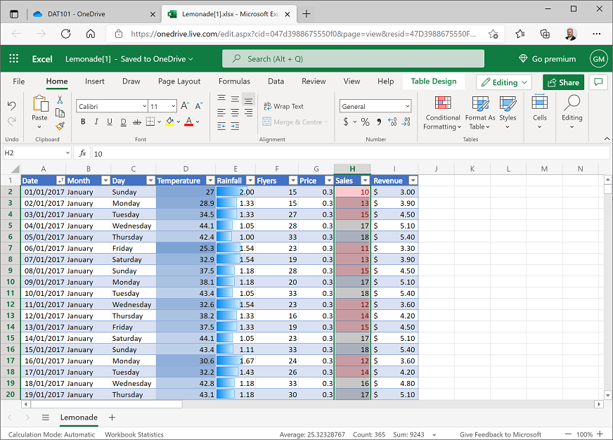
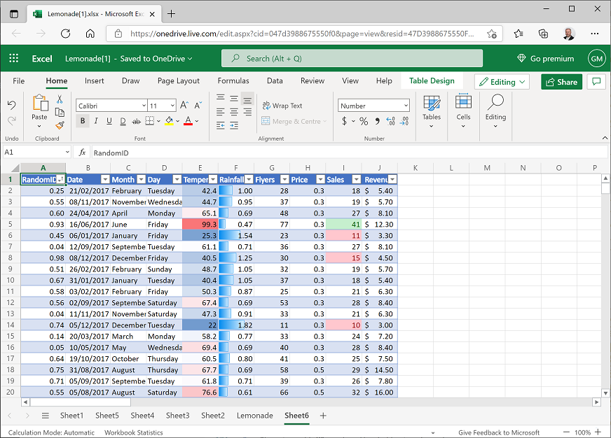
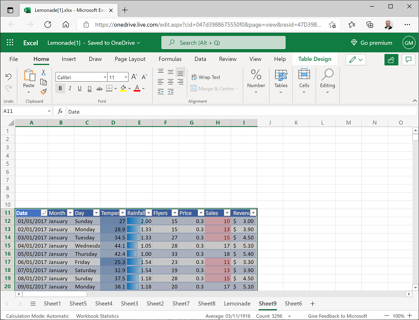
If you have not already done so, in your web browser, navigate to https://onedrive.live.com, and sign in using your Microsoft account credentials. Then open the Lemonade.xlsx workbook in the folder where you uploaded it in the previous labs and view the Lemonade worksheet. Your workbook should look like this:
In cell K1, enter the text Sales Statistics, and format it as bold.
In cell K2, enter the text Mean, and then select cell L2, and enter the following formula in the fx bar:
```
 =AVERAGE(H2:H366)
```
This calculates the arithmetic mean for sales, which should be slightly over 25.3.
In cell K3, enter the text Median, and then select cell L3 and enter the following formula:
```
 =MEDIAN(H2:H366)
```
This calculates the median for sales, which should be 25.
In cell K4, enter the text Mode, and then select cell L4 and enter the following formula:
```
 =MODE.SNGL(H2:H366)
```
This calculates the mode for sales, which should also be 25.
In cell K5, enter the text Variance, and then select cell L5 and enter the following formula:
```
 =VAR.P(H2:H366)
```
This calculates the variance for sales, which should be slightly over 47.39.

Note that the formula for variance in this case applies to the full population of data, hence the .P extension in the function name – you’ll explore working with data samples later in this lab.
In cell K6, enter the text Std Dev, and then select cell L6 and enter the following formula:
```
 =STDEV.P(H2:H366)
```
This calculates the standard deviation for sales, which should be slightly over 6.88.

Note once again that the formula for standard deviation in this case applies to the full population of data.

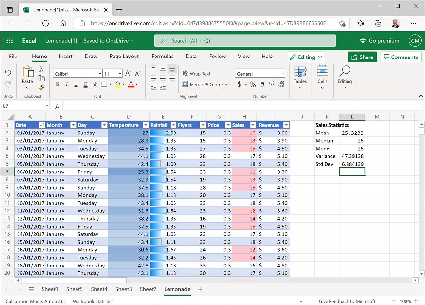
Your worksheet should now look like this:

The statistics you have calculated tell you something about the distribution of the sales values, but it can often be easier to visualize the data to get a sense of how the data is distributed.

Visualize the distribution of sales values

Select all the data in the Sales column, including the header. Then on the Insert tab of the ribbon, in the Other Charts drop-down list, click the Histogram chart (which is the first one in the Statistical section).
Select the chart that is produced and edit the chart title to change it to Sales. Then move the chart so that it is to the right of the statistics you calculated in the previous exercise. The chart should look like this:
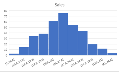
Examine the chart, and note the following:
- The histogram shows the frequency of different values for Sales values grouped into ranges, or bins. For example, there are around 15 days with a Sales value between 10.4 and 13.8; and there are around 20 days with a Sales value between 34.2 and 37.6.
- The most frequently occurring Sales values are between 24 and 27.5. This range includes the mean, median, and mode statistics you calculated previously. In other words, on most days, the number of sales was more or less in the middle of the lowest and highest selling days.
- The distribution is approximately symmetrical around the middle values, forming a “bell-shaped curve” that tapers evenly towards the ends; where there are few occurrences of extreme values for Sales. Statisticians refer to this kind of distribution as a normal distribution.
- The standard deviation you calculated previously is just under 6.9. This statistic provides a standard unit of variance around the mean (which is just over 25.3). The data within 1 standard deviation above or below the mean) therefore includes values from approximately 18.4 to around 32.2, as shown here:
  
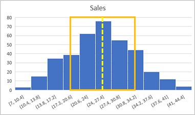
  In a normal distribution, around 68.26% of the data falls within a single standard deviation; so in this case, the number of sales was between 18.4 and 32.2 on 68.26% of the days. Around 95.45% of values fall within 2 standard deviations in a normal distribution, so there were between 11.5 and 39.1 sales on 95.4% of days.
Select all the data in the Sales column, including the header. Then on the Insert tab of the ribbon, in the Other Charts drop-down list, click the Box and Whisker chart (which is the third one in the Statistical section).
Select the chart that is produced and edit the chart title to change it to Sales. Then move the chart so that it is to the right of the histogram you created previously. The chart should look like this:
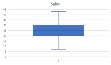
Examine the chart, and note the following:
- The horizontal line in the middle indicates the median value for sales. This is the 50% percentile – in other words, 50% of the values are higher than this, and 50% are lower.
- The X in the box indicates the mean – this is only slightly higher than the median.
- The filled box indicates the range of values in the second and third quartiles – in other words, from the 25th percentile to the 75th percentile. These values range from around 20 to 30, indicating that the number of sales on half of the days was within this range,
- The lines extending from the box (known as whiskers) show the range for the first and fourth quartiles, on which there were more or fewer sales than in the second and third quartiles.

Analyze statistics for rainfall

Leave some space under the existing statistics, and in cell K17, enter the text Rainfall Statistics, and format it as bold.
In cell K18, enter the text Mean, and then select cell L18 and enter the following formula:
```
 =AVERAGE(E2:E366)
```
This calculates the arithmetic mean for rainfall, which should be 0.83.
In cells K19 to L22, calculate the median, mode, population variance, and population standard deviation for rainfall, in the same way you did for sales previously. When you’re finished, your worksheet should look like this:

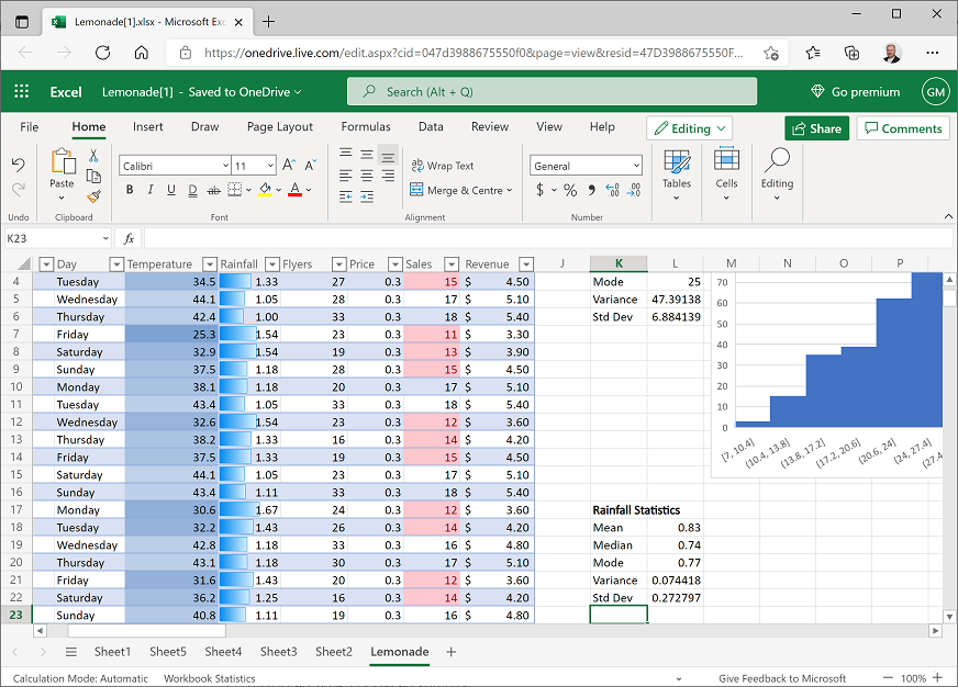
Note that the mean rainfall is quite a bit higher than the median and mode.
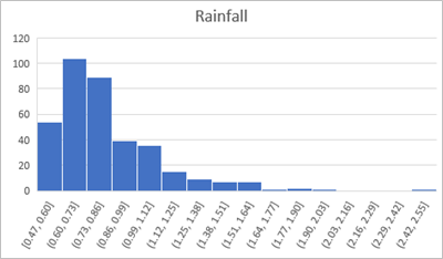
Create a histogram of rainfall, and then add an appropriate chart title and move the chart to the right of the rainfall statistics. The rainfall histogram should look like this:
Examine the histogram and note that the distribution of the rainfall data is not normal.

The median value is around 0.74, so on half the days there was less rain than this, and on half there was more; however, on a rare few days, there was much more rain than this - as much as 2.42 to 2.55. These infrequent days of extremely high rainfall are skewing the distribution by “pulling” the mean to the right. This results in a long tail of infrequently occurring values that tapers towards the right. We therefore refer to this as a right-skewed distribution (had the tail pulled the mean to the left, it would be a left-skewed distribution).
Create a box and whisker chart of rainfall with an appropriate title; and move it to the right of the rainfall histogram. The box and whisker chart should look like this:
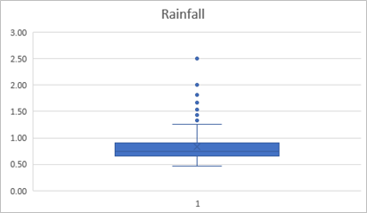
Examine the chart and note the following:
- The line indicating the median (50th percentile) noticeably lower than the X indicating the mean.
- The filled box, representing the 2nd and 3rd quartiles represents 50% of the data – in other words, on half of the days, the rainfall was between around 0.6 and 0.8.
- The dots indicate outliers; rare values that are considered extreme compared to the typical range of values, which lies within the whiskers.
- Even discounting the outliers, the range of values in the 4th quartile is larger than that of the other quartiles.

Challenge: Analyze temperature statistics

Calculate the mean, median, mode, population variance, and population standard deviation of temperature.
Create a histogram and a box and whiskers chart for temperature to visualize the distribution.

Exercise 2: Working with Samples

Until now, we’ve worked with the full population of data – in other words, we had all of Rosie’s lemonade sales data to work with. In reality, it’s more usual to work with a sample of data. For example, suppose you needed to conduct some research to determine the most common eye color in the US. It would be unrealistic to examine the eyes of every person in the US, so you would approach this problem by surveying a representative sample of people, and use the statistics collected as approximations for the full population parameters.

Create a random sample

On the Lemonade worksheet, select in cell A1 and then press CTRL+A (⌘ + A on Mac OSX) to select the entire table of lemonade sales data. Then on the Home tab of the ribbon, click Copy.
Add a new worksheet to the workbook and click cell A1 of the new worksheet. Then on Home tab of the ribbon, click Paste to paste the copied table into the new worksheet (this may take a few seconds).
Click cell A1 (the Date header), and then on the Home tab of the ribbon, in the Cells section, click the Insert drop-down list and select Insert Table Columns to the Left. This inserts a new column for a table field named Column1.
In the new cell A1, rename Column1 to RandomID, and then select column A and in the format drop-down list in the Number section of the Home tab of the ribbon (which should currently have General selected), click Number.
In cell A2, enter the following formula:
```
 =RAND()
```
This will generate random numbers in the RandomID column.
Click the drop-down arrow in the RandomID column header and click Sort Smallest to Largest. The data in the table is sorted by the RandomID field, which randomizes the order of the data records. This makes it easier to select a random sample of records (a random sample is more likely to be representative of the population than a sample that is based on some inherent order in the data itself). Your worksheet should now look like this:
In Cell M1, enter the text Mean Rain, and in cell N1 enter the text Rain StDev.
In cell L2, enter the text Population.
Select cell M2 and enter the following formula:
```
 =AVERAGE(F2:F366)
```
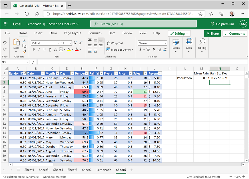
Select cell N2 and enter the following formula:
```
=STDEV.P(F2:F366)
```
This gives you full population parameters for the mean and standard deviation of rainfall, so you can compare them with sample statistics.

Your workbook should now look like this:
In cell L3, enter the text Sample1.
Select cell M3 and enter the following formula:
```
=AVERAGE(F2:F41)
```
Select cell N3 and enter the following formula:
```
=STDEV.S(F2:F41)
```
This gives you sample statistics for the mean and standard deviation of rainfall based on the first 40 random rows of data. Note that you use the same AVERAGE function to calculate a sample mean or population mean, but you use the STDEV.S function to calculate the standard deviation for a sample – this incorporates some additional variance to allow for sample bias. Your spreadsheet should now look similar to this (the figures may not be exactly the same because of the randomization of the data):

Compare the sample statistics with the population parameters.
In cell L4, enter the text Sample2.
Select cell M4 and enter the following formula:
```
=AVERAGE(F35:F74)
```
Select cell N4 and enter the following formula:
```
=STDEV.S(F35:F74)
```

This produces statistics from a different sample. Note that the closeness of the sample statistics to the population parameters varies depending on the sample. In this case, both samples include 40 observations - using larger samples generally results in statistics that are closer to their actual population parameters.

Create a sampling distribution

Select cells L3 to N4 (the Sample1 and Sample2 statistics you created previously; but not the population parameters), and then drag the small square handle (▪) at the bottom right of the selected cells down to row 292. This creates 290 samples as shown here:

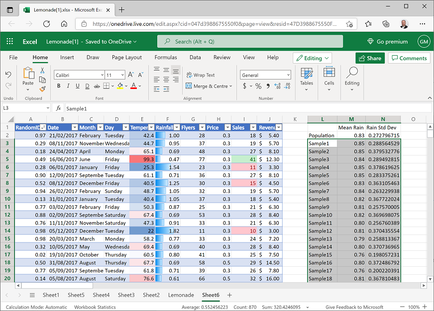
The means of the samples form a sampling distribution of the mean – in other words, a new data distribution that consists of the sample means.
In cell O1, enter the text Sampling Mean. Then select cell O2 and enter the following formula:
```
 =AVERAGE(M3:M292)
```
This calculates the mean of the sample means; in other words, the mean of the sampling distribution. This should be fairly close to the population mean as shown here (yours may not be exactly the same as the population mean, but it should be close!)
Select cell M3 (the Sample1 mean) and then hold the Shift and Ctrl keys and press the Down-Arrow key to select all the other sample means (if you are using a Mac OSX computer, hold the Shift and ⌘ keys, and press the Down-Arrow key).
In the Insert tab of the ribbon, in the Other Charts drop-down list, select Histogram (the first chart in the Statistical section) and view the histogram that is created, as shown here (your chart may look a little different):

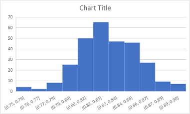
The histogram may not look exactly symmetrical; but when you create a sampling distribution from a sufficiently large number of reasonably-sized samples, you’ll find that it has a bell-curved appearance. We won’t discuss this any further in this course, but it’s useful to know that with enough random samples, a sampling distribution generally takes on a normal distribution due to something called the central limit theorem – even when (as in this case), the population data from which the sample means are derived is not normally distributed.

Challenge: Analyze temperature samples

Create a sampling distribution based on 290 samples of mean Temperature. Each sample should be based on 40 random observations.
Calculate the mean of the temperature sampling distribution.

Exercise 3: Inferential statistics and hypothesis testing

So far, we’ve explored descriptive statistics that describe the distribution of data in a full population or a sample. Inferential statistics, as the name suggests, are used to make inferences, or predictions, from data based on statistical relationships between fields (or features) of the data.

Measure correlation

Switch back to the Lemonade worksheet in the Lemonade.xlsx workbook and select cell A1 (the Date column header).
On the Insert tab of the ribbon, click PivotTable; and insert a PivotTable for the lemonade sales table into a new worksheet.
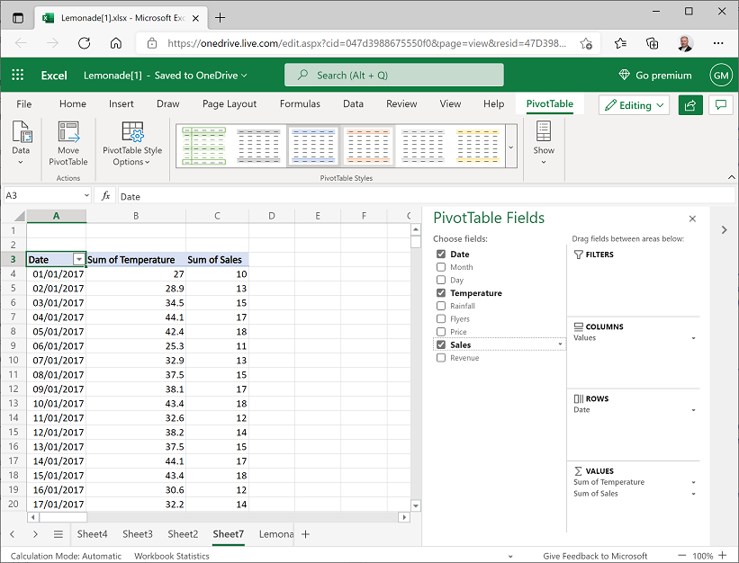
In the PivotTable Fields pane, drag Date to the Rows area and drag Temperature and Sales to the Values area so that your worksheet looks like this:
Scroll to the bottom of the PivotTable until you can see the Grand Total row. You need to copy the temperature and sales values, excluding this grand total to a new worksheet.
Click the cell containing the temperature value for December 31 2017 (above the grand total). Then press SHIFT + CTRL + ⇧ (SHIFT + ⌘ + ⇧ on Mac OSX) to select the column of temperature values, and then press SHIFT + ⇨ to extend the selection to include the sales values. Finally, use the 🗐 button on the Home tab of the ribbon to copy the selected cells to the clipboard.
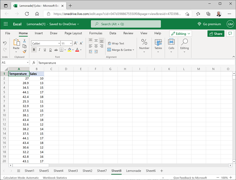
Create a new worksheet, and then on the new worksheet click cell A1 and use the Paste button (📋) to paste the copied data. Then change the columns headers to Temperature and Sales as shown here:
Select cell A1 (the Temperature column header) and press CTRL + A (⇧ + A on Mac OSX) to select the data, and then on the Insert tab of the ribbon, in the Scatter drop-down list, click the first scatter plot. This inserts a scatter plot that looks like this:

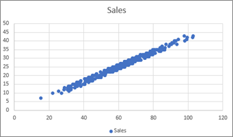
Note that the scatter plot seems to reflect a linear relationship between temperature and sales, in which the higher the temperature, the more sales there are.
Move the chart to the side of the worksheet to create some space, and in cell D1, enter the text Correlation. Then select cell D2, and enter the following formula in the fx bar:
```
 =CORREL(A2:A366,B2:B366)
```
This calculates the correlation between temperature and sales; and should produce a value of around 0.989832. Correlation is a statistical measurement of the strength of an apparent relationship between two numeric variables – in this case, temperature and sales.

Your worksheet should look like this:

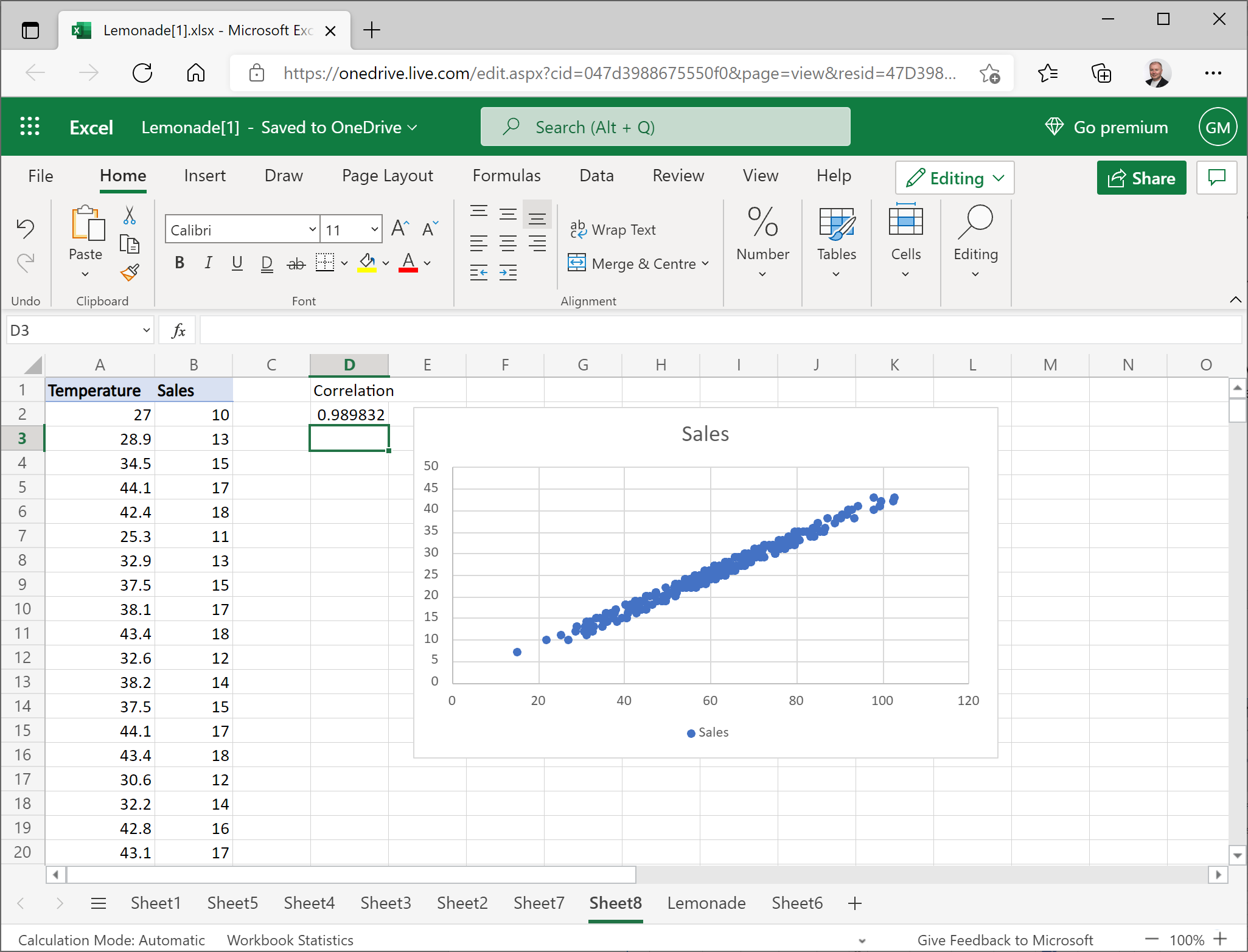
Correlation is measured as a value between -1 and 1. A value close to 1 indicates a positive correlation; in other words, high values for one variable seem to correspond with high values for the other variable. A value close to -1 on the other hand indicates a negative correlation, in which high values for one variable correspond to low values for the other variable. A value close to 0 indicates the lack of any discernible relationship between the variables.

With a correlation of almost 0.99, there is a strong positive relationship between temperature and sales.

Note: Statisticians often quote the mantra “correlation is not causation”. We can use correlation to determine that days with high sales volumes tend to have high temperatures; but we can’t say that Rosie sold a lot of lemonade on a particular day because the temperature was high – just as we can’t say that a day was particularly hot because Rosie sold a lot of lemonade. In fact, there could be a “hidden” third factor that affects both sales of lemonade and temperature. For example, during the summer months, when lemons are in season, the temperature tends to be higher.

Challenge: Calculate rainfall / sales correlation

Calculate the correlation between Rainfall and Sales.
What does the correlation indicate?

Conduct a Hypothesis Test

On the Lemonade worksheet, clear any filters from the table of lemonade sales data. Then click in cell A1 and then press CTRL+ A (⌘ + A on Mac OSX) to select the entire table of lemonade sales data and copy it to the clipboard.
Add a new worksheet to the workbook and paste the copied data into cell A11 of the new worksheet (leaving ten blank rows above the pasted data), like this:

You have hypothesized that on days where Rosie distributes a higher than average number of flyers, sales are higher. You need to test this hypothesis to determine if any increase in sales on days with higher than average flyer distribution can be explained by chance, or if the variation in sales is too improbable to be explained by chance alone. To help determine this, you need to create a data sample containing sales for days with higher than average flyer distribution.
In the drop-down list for the Flyers column header, in the Number Filters sub-menu, click Above Average.
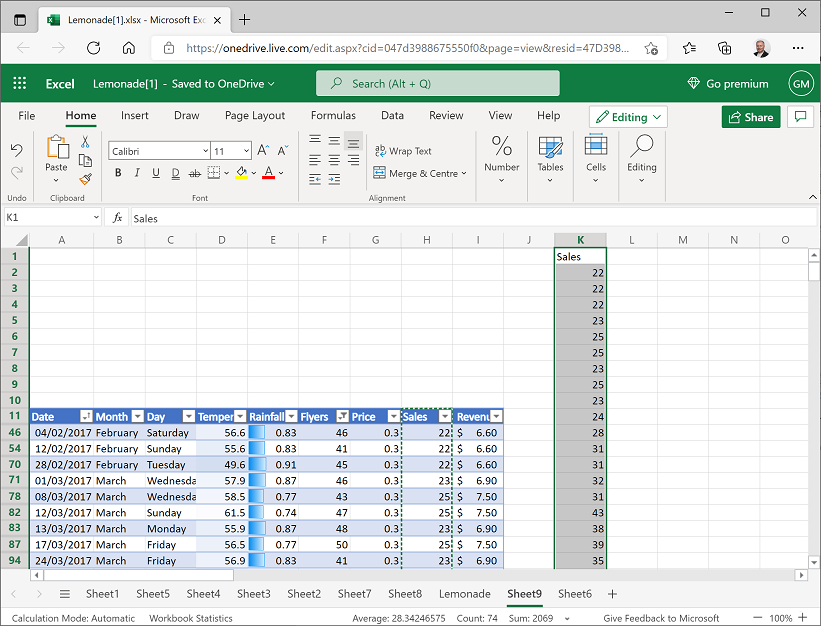
Select and copy the Sales column (including the header), and then select cell K1 and in the Paste (📋) drop-down list, click Paste Values. This pastes the filtered sales data sample (which contains the observations from days with higher than average flyer distribution) as shown here:
Clear the filter from the Flyers column so that the table starting in row 11 shows the full population of sales data.
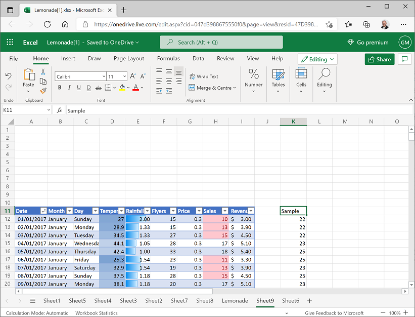
Select the sample data (including the header) and move it to cell K11, then In cell K11, change the column header to Sample as shown here:
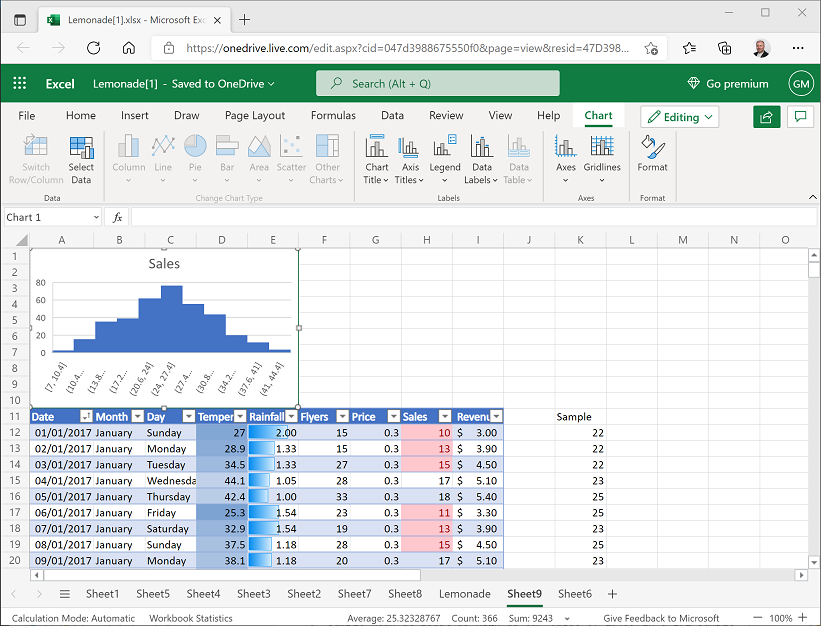
Select the Sales column of data (including the header), and insert a histogram showing the distribution of sales. Change the chart title to Sales, and then resize and position the histogram in the space above the data, like this:
In cell G2, enter the text Mean, and then select cell H2 and enter the following formula to calculate the mean sales value for all of the data:
```
 =AVERAGE(H12:H376)
```
In cell G3, enter the text StDev, and then in cell H3 enter the following formula to calculate the standard deviation for all sales values:
```
=STDEV.P(H12:H376)
```
In cell G4, enter the text Sample, and then in cell H4 enter the following formula to calculate the sample mean of sales for days with higher than average flyer distribution (of which there are 172):
```
=AVERAGE(K12:K183)
```
In cells G2 to H4, you should now have the following values:
- Mean: 25.32329
- StDev: 6.884139
- Sample: 29.99419
From this, you can see that the sample mean of approximately 29.99 (the mean number of sales on days with higher than average flyer distribution) is indeed greater than the population mean of around 25.32 (the mean number of sales on all days). You can also see in the histogram that the population mean is in the middle, and the sample mean is to the right. However, there is some variance in the population data resulting in a standard deviation of around 6.88. So can the higher sales on days where Rosie distributed more flyers be explained simply by this normal variance (we’ll call this our null hypothesis), or is there enough evidence to reject that explanation in favor of an alternative hypothesis that the sales increase on these days is statistically significant enough to have been caused by something other than random chance?

To determine this, we’ll conduct something called a Z-Test.
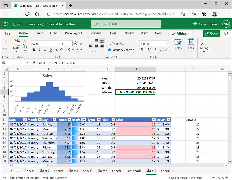
In cell G5, enter the text P-Value, and then select cell H5 and enter the following formula:
```
=Z.TEST(K12:K183, H2, H3)
```
This calculates a p-value, which is the probability of observing a sample mean at least as high as our value of 29.99 in a 172 sample distribution from a population with a mean of 25.32, and a standard deviation of 6.88.
The p-value is probably displayed in scientific notation, with a value similar to 2.83128E-19. To view this as a regular decimal number, select the p-value (in cell H4) and on the Home tab of the ribbon, in the Number section select the Number format and then repeatedly click the Increase Decimal (^←0_.00) button until the first non-zero decimal place is shown. It should be close to 0.0000000000000000003, as shown here:

This is clearly a very small probability, and in fact it is common to use a value of 0.05 (or 5%) as the threshold for rejecting the null hypothesis in favor of the alternative hypothesis. So in this case, the p-value is much lower than this threshold and we can reject the null hypothesis that the increase in sales can be explained by random variance and conclude that there is some non-random factor at work here. Note that we can’t categorically say that the increase in sales is because of the higher number of flyers distributed; but we can say that on the days where more leaflets were distributed, there was a statistically significant increase in sales.

It’s worth briefly thinking a little bit about what this means. What does this show? We have shown that, had the results been due to chance (i.e., H0 = true), we could possibly still get these results. In other words, we haven’t disproven chance as an explanation. However, we showed that the probability of getting these results is very, very, very small…only 0.0000000000000000003. We are safe in rejecting chance as an explanation for our results here.

There’s a lot more to hypothesis testing than we have room to discuss here. The example above is a one-sample test (it tests a single sample of data to compare the sample mean with a hypothesized mean). The example is also a one-tailed test, and in this case, the test is right-tailed (our p-value describes the probability of a sample mean being significantly higher than the hypothesized mean, which means the critical area for rejection of the null hypothesis is under the right tail of a normal distribution curve.

You can also use the Excel Z.TEST function to perform a two-tailed test, in which the alternative hypothesis is that the sample mean is not equal to the hypothesized mean (so there are critical areas under both the right and left tails of the normal distribution curve). To perform 2-tailed tests in Excel, you need to manipulate the value retuned by the Z.TEST function to calculate the correct p-value as follows:
```
= 2*MIN(Z.TEST(SampleRange, HypothesizedMean [,PopStDev]), 1–Z.TEST(SampleRange, HypothesizedMean [,PopStDev]))
```
For more information about using the Z.TEST function in Excel, see the Excel documentation.

Challenge: Test rainfall hypothesis

Test the following hypotheses:
- H0 (null hypothesis): Higher mean sales on days with lower than average rainfall can be explained by random variance.
- H1 (alternative hypothesis): Mean sales on days with lower than average rainfall are significantly higher than the population mean and can’t be explained by random variance.
You should reject the null hypothesis if the p-value for your test is less than 0.05.

< Back

Next >